Facade design: The benefits of early-stage energy modelling
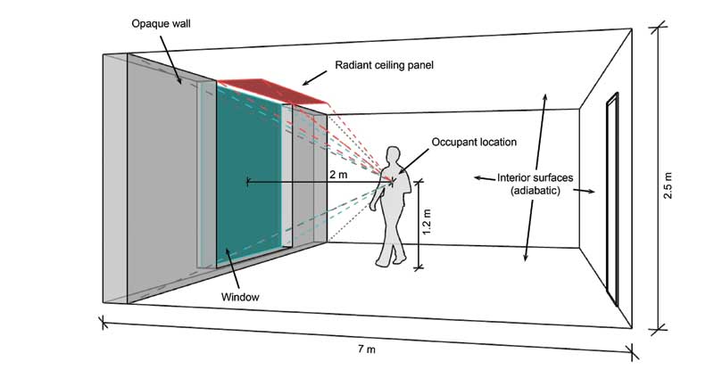
The simplicity of the model’s inputs is a result of the underlying calculation methodologies. (Figure 1) Most of the equations used in the Python script are calculated by hand. For example, the inside surface temperature of the facade is calculated using Fourier’s law of 1D steady-state conduction. The effect of solar radiation on the window surface temperature is approximated using SHGC and Tsol.4 View factors, which are necessary for computing the mean radiant temperature (MRT), are calculated using geometric solid angle formulas.5 Ventilation heat losses are calculated using the familiar formula, Q = mcΔT, which only requires knowledge of the ventilation rate, inside-outside temperature difference, and the volumetric heat capacity of air. The advantage of implementing these basic methods in a computer script (opposed to performing the calculations by hand or in Excel), is a user can efficiently analyze multiple facade options, at an hourly timestep, with minimal inputs.
From outputs to insights
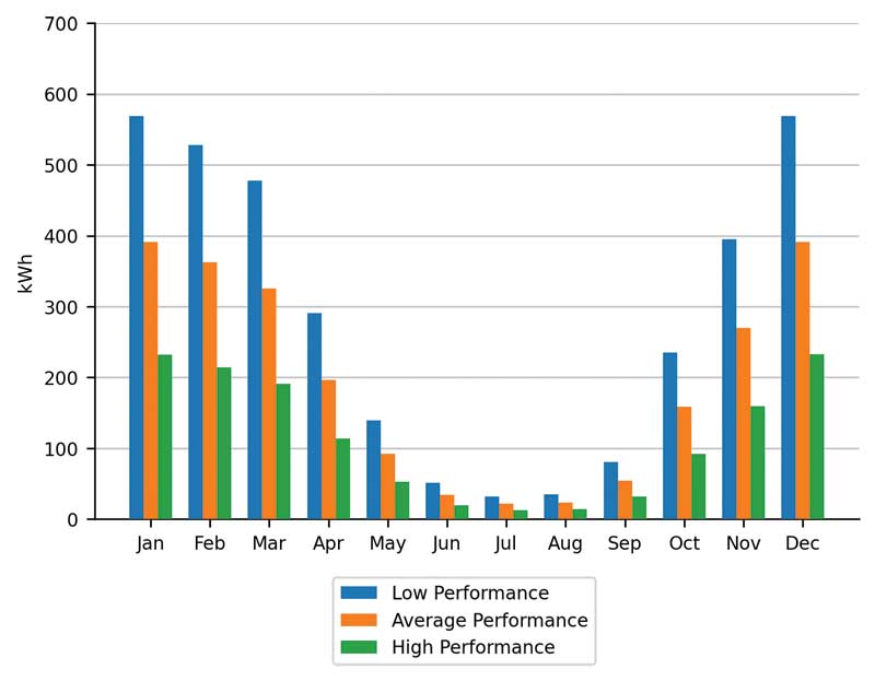
With some data processing and visualization, the model’s raw outputs are transformed into useful insights. Comparisons of the energy performance achieved by various facade options are especially useful during the early stages of design. For example, a comparison of monthly heating demand can show exactly when a higher performance facade is expected to generate the most energy savings. Figure 2 compares a low, average, and high-performance facade applied to a multi-unit residential building in Toronto. It is clear the high-performance facade would be most impactful during the winter.
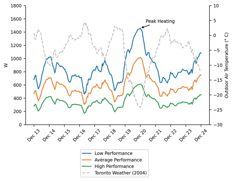
A comparison of the hourly heating load can show how the building would respond to an extreme weather event, and if certain facades preclude the use of certain mechanical equipment (e.g. low temperature hot water systems). Figure 3 shows how the heating load on a radiant ceiling panel would respond to a cold snap in Toronto. The peak loads for the low performance and high-performance facades—1000 W and 600 W respectively—were determined to be within the capacity of the considered equipment.
Most importantly, a comparison of TEDI can help an architect understand which facades put the building on track to achieve green building certifications, such as TGS or Passive House. Figure 4 (page 3) compares three facade options across four compass orientations (North, East, South, West) and two glazing ratios (40 per cent and 80 per cent). Only the high performance, 40 per cent glazing options came close to the Passive House standard. Only the low performance, 80 per cent glazing options fared worse than TGS’s minimum requirement for residential buildings.
The Python script automatically generates these comparisons and accompanying charts, making it convenient to assess multiple facade options simultaneously. The script can also create more “visual” outputs, such as a spatial heat map of the operative temperatures in a room. These types of outputs can be useful for explaining how the energy required to maintain thermal comfort varies with facade performance. The example on page 3 (Figure 5) considers a radiant ceiling panel installed above a window of varying thermal performance. It is clear the mechanical system has to work harder to compensate for the low-performance window when compared to the high-performance window.
Sign up for our weekly newsletter
Construction Canada weekly newsletters give the latest AEC industry news for those who build, design, engineer, specify, renovate or operate in the built environment.
Related Products & Services
Read the Latest Issue